Examples
Some brief examples of regression and classification using I-priors. All error terms \(\epsilon\) are assumed to be normally distributed, as per (1), unless specified otherwise.
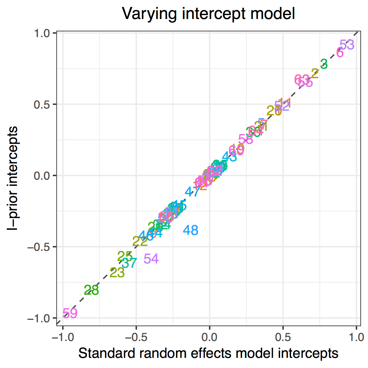
Multilevel Analysis of Pupils’ GCSE Scores
Aim: Obtain estimates for random intercepts and slopes for a multilevel data set, and compare with standard random effects model estimates.
Data: GCSE scores (\(y_{ij}\)) for 4,059 pupils at 65 inner London schools (\(j\)), together with their London reading test results (\(x_{ij}\)).
Model:
\[y_{ij} = f_1(x_{ij}) + f_2(j) + f_{12}(x_{ij}, j) + \epsilon_{ij}\]with \(f_1\) in the canonical RKHS, \(f_2\) in the Pearson RKHS, and \(f_{12}\) in the tensor product space.
Results: Good agreement between I-prior estimates and standard random effects model estimates.

Longitudinal Analysis of Cattle Growth
Aim: Discern whether there is a difference in the two treatments given to the cows, and whether this effect varies among individual cows.
Data: A balanced longitudinal data set of weight measurements \(y_{it}\) for 60 cows (\(x_{1it}\)) at different time points \(t = 1,\dots,11\). Half of the herd were randomly assigned to treatment group A, and the other half to treatment group B.
Model: Assume a smooth effect of time and nominal effect of cow index and treatment group:
\[y_{it} = f_1(x_{1it}) + f_2(x_{2it})+ f_3(t) + f_{13}(x_{1it}, t) + f_{23}(x_{2it}, t) + f_{123}(x_{1it}, x_{2it}, t) + \epsilon_{it}\]with \(f_1\) and \(f_2\) in the Pearson RKHS, \(f_3\) in the fBm-0.5 RKHS, and the interaction functions in the appropriate tensor product space. This model can be succintly represented as
\[y_{i} = f_{1t}(x_{1it}) + f_{2t}(x_{2it})+ f_{12t}(x_{1it}, x_{2it}) + \epsilon_{i}.\]Results: Four models were fitted, and the results tabulated below.
| Explanation | Model | Log-lik. | No. of param. | |
|---|---|---|---|---|
| 1 | Growth due to cows only | \(f_{1t}\) | -2792.2 | 3 |
| 2 | Growth due to treatment only | \(f_{2t}\) | -2295.2 | 3 |
| 3 | Growth due to both cows and treatment | \(f_{1t} + f_{2t}\) | -2270.9 | 4 |
| 4 | Growth due to both cows and treatment, with treatment varying among cows | \(f_{1t} + f_{2t} + f_{12t}\) | -2250.9 | 4 |
To test for a treatment effect, we test the signifiance of the scale parameter for the treatment variable in Model 2 (p-value < 10-6). To test whether treatment effect differs among cows, we compare likelihoods for Models 3 and 4.
Predicting Fat Content of Meat Samples from Spectrometric Data
Aim: Predict fat content of meat samples from its spectrometric curves (Tecator data set).
Data: For each meat sample, 100 channel spectrum of absorbances (\(x_i \in \mathbb R^{100}\)) together with the contents of moisture, fat (\(y_i\)) and protein measured in percent. 160 samples were used to train the model, and 55 were used for testing.
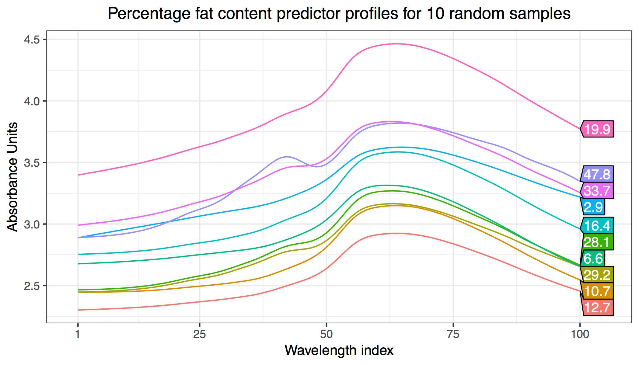
Model: Take first differences of \(x\) (see here for an explanation) and obtain \(z_i \in \mathbb R^{99}\). We then assume various effects of \(z_i\) on \(y_i\) using the linear, polynomial (quadratric and cubic) and fBm (smooth).
Results: Training and test errors are tabulated below. The smooth I-prior model outperforms methods such as Gaussian process regression (13.3), kernel smoothing (1.85), single index models (1.18) and sliced inverse regression (0.90) in test error rates.
| Model | Training error | Test error | |
|---|---|---|---|
| 1 | Linear | 2.85 | 3.24 |
| 2 | Quadratic | 0.72 | 1.23 |
| 3 | Cubic | 0.99 | 1.65 |
| 4 | Smooth (fBm-0.5) | 0.00 | 0.67 |
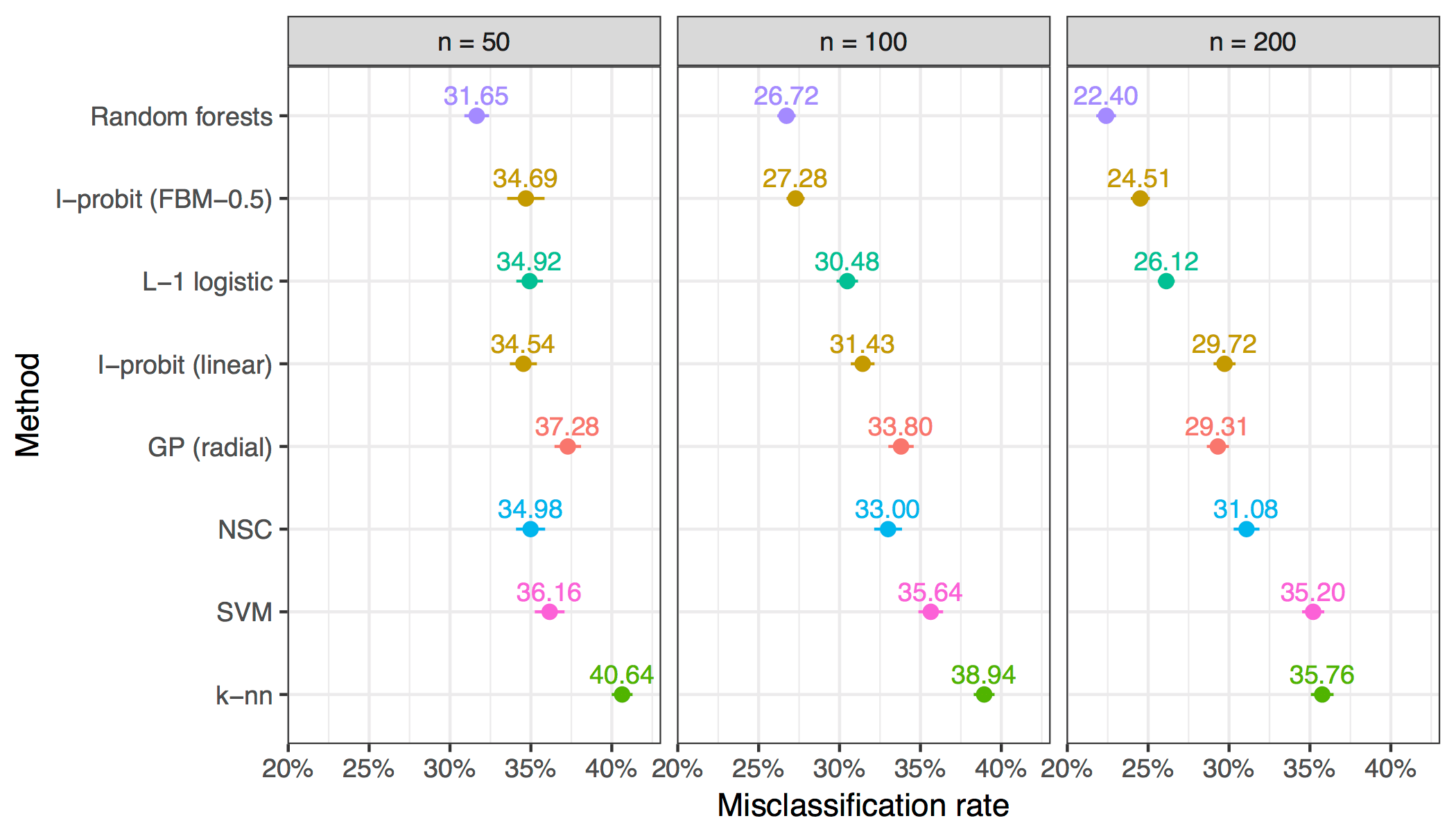
Diagnosing Cardiac Arrhythmia
Aim: Predict whether patients suffers from a cardiac disease based on various patient profiles such as age, height, weight and a myriad of electrocardiogram (ECG) data.
Data: 451 observations of 279 predictors and binary variables indicating whether each patient had arrhythmia or not. All 279 predictors are continuous, and they were standardised beforehand.
Model: A binary I-probit model using the linear and fBm-0.5 kernel to predict the probability of having cardiac arrhythmia:
\[p_i = \Phi\big(f(x_i)\big)\]where \(f\) lies in either the canonical or fBm-0.5 RKHS. Since the variables \(x_i \in \mathbb R^{279}\) were standardised, it is sufficient to use a single scale parameter.
Results: In order to test predictive performance, the data was randomly split into training sets of sizes 50, 100, and 200, with the remaining forming the test set. The model was fitted and out-of-sample misclassification rates noted. This was then repeated 100 times to obtain averages and standard errors.
The I-probit models outperformed some of the more popular classifiers, including Gaussian process classification, nearest shrunken centroids, support vector machines and \(k\)-nearest neighbours.
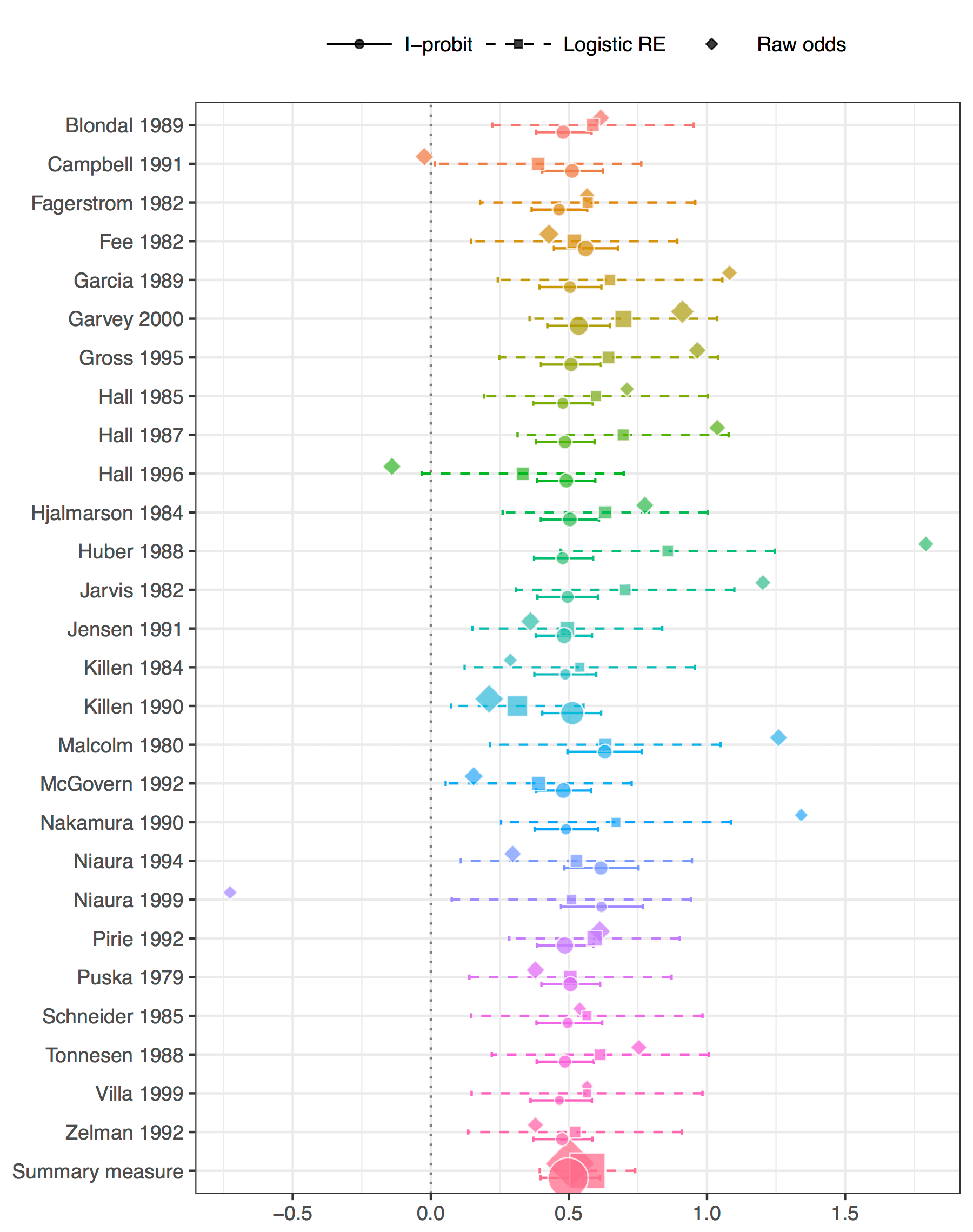
Meta-analysis of Smoking Cessation
Aim: Inference on the effect size of nicotine gum treatment on smoking cessation based on data from multiple, independent studies.
Data: Records of whether each of the 5,908 patients in 27 separate studies (\(j\)) successfully quit smoking (\(y_{ij}\)) and also whether they were subjected to actual treatment or placebos (\(x_{ij}\)).
Model: The Bernoulli probabilities \(p_{ij}\) for each patient \(y_{ij}\) are regressed against the treatment group indicators \(x_{ij}\) and each patients’ study group \(j\) via the probit link:
\[p_i = \Phi\big(f_1(x_{ij}) + f_2(j) + f_{12}(x_{ij}, j)\big)\]where \(f_1\) and \(f_2\) lie in the Pearson RKHS, and \(f_{12}\) in their tensor product space.
Results: Fitted model probabilities were obtained, and log odds ratios calculated and compared against the standard logistic random effects model.
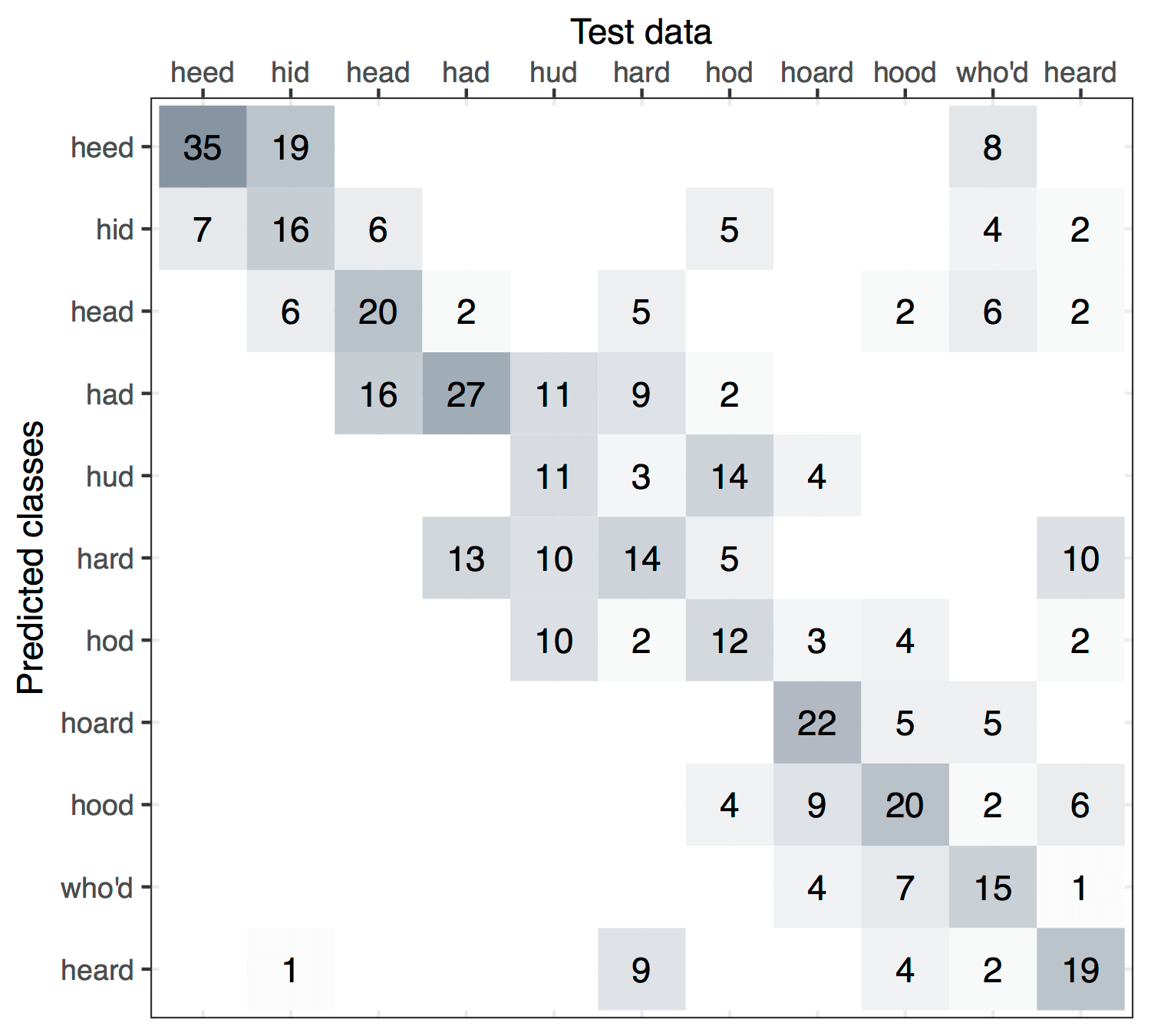
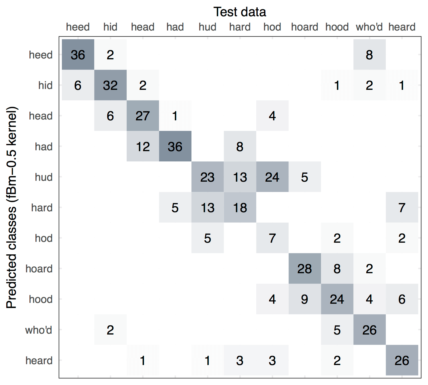
Vowel Recognition in Speech Recordings
Aim: Multiclass classification of Deterding’s vowel data set, in which the task is to correctly associate digitised speech recordings with the specific vowel used for that speech.
Data: Multiple speakers, male and female, uttered 11 vowels each and their speech recorded. These were then processed using speech processing techniques. The result is 990 data points consiting of a ten-dimensional numerical predictor \(x_i\) and also the class of vowel for each data point \(y_i\). These were split roughly equally into a training and test set.
Model: A multinomial I-probit model to predict the class probabilities for each data point:
\[p_{ij} = g_j^{-1} \big( f(x_i) \big)\]where \(f_j\) lies in either the canonical or fBm-0.5 RKHS for each class \(j \in \{1,\dots,11\}\) and \(g^{-1}\) is the function as described here. The predicted class is given by \(\hat y_i = \arg\max_j p_{ij}\).
Results: Out-of-sample misclassification rates for the fBm I-prior model was the best among several methods which include logistic regression, linear and quadratic discriminant analysis, decision trees, neural networks, nearest neighbours, and flexible disciminant analysis. While the canonical I-probit did not fare as well, it did however gave improvement over linear regression.
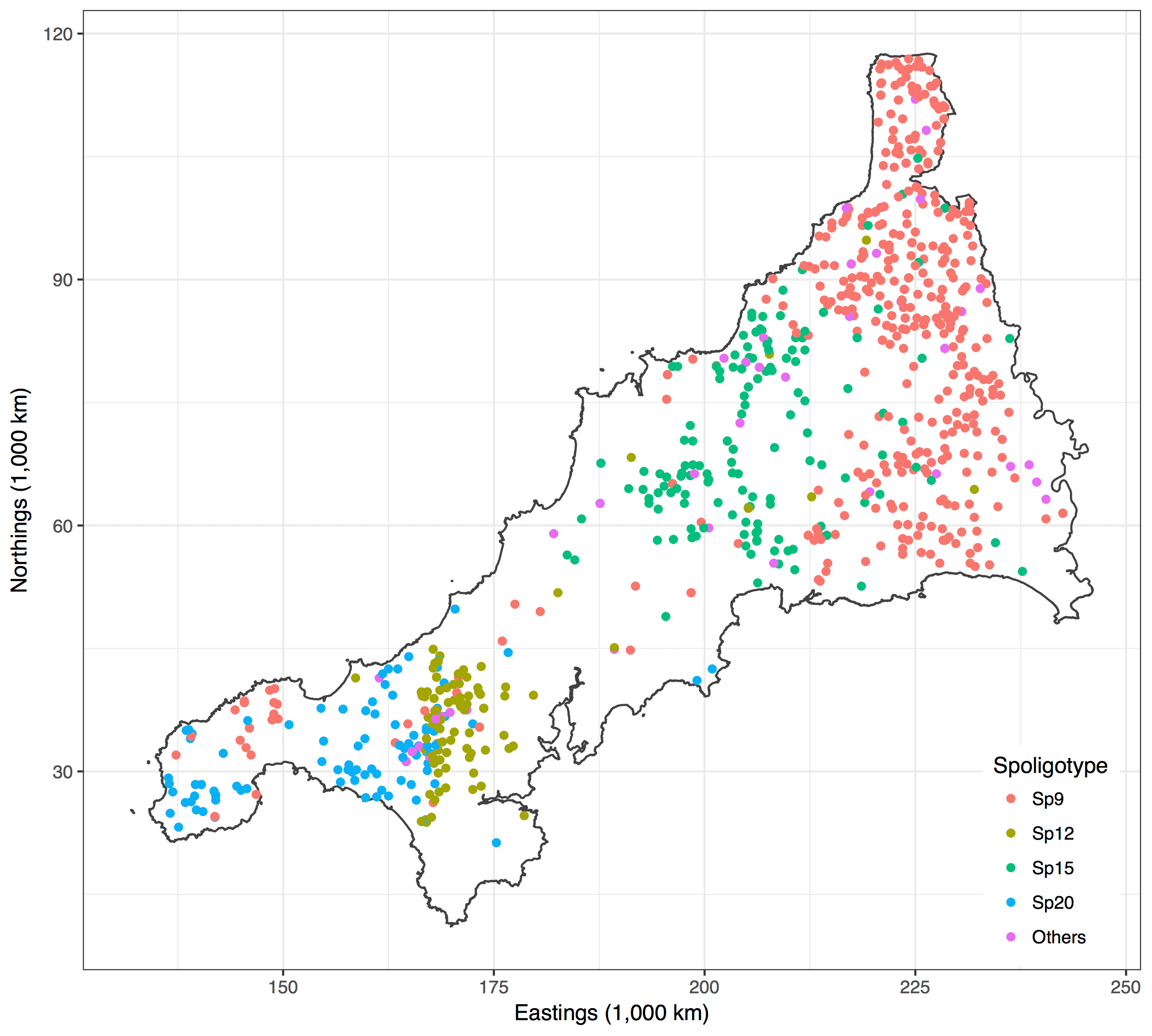
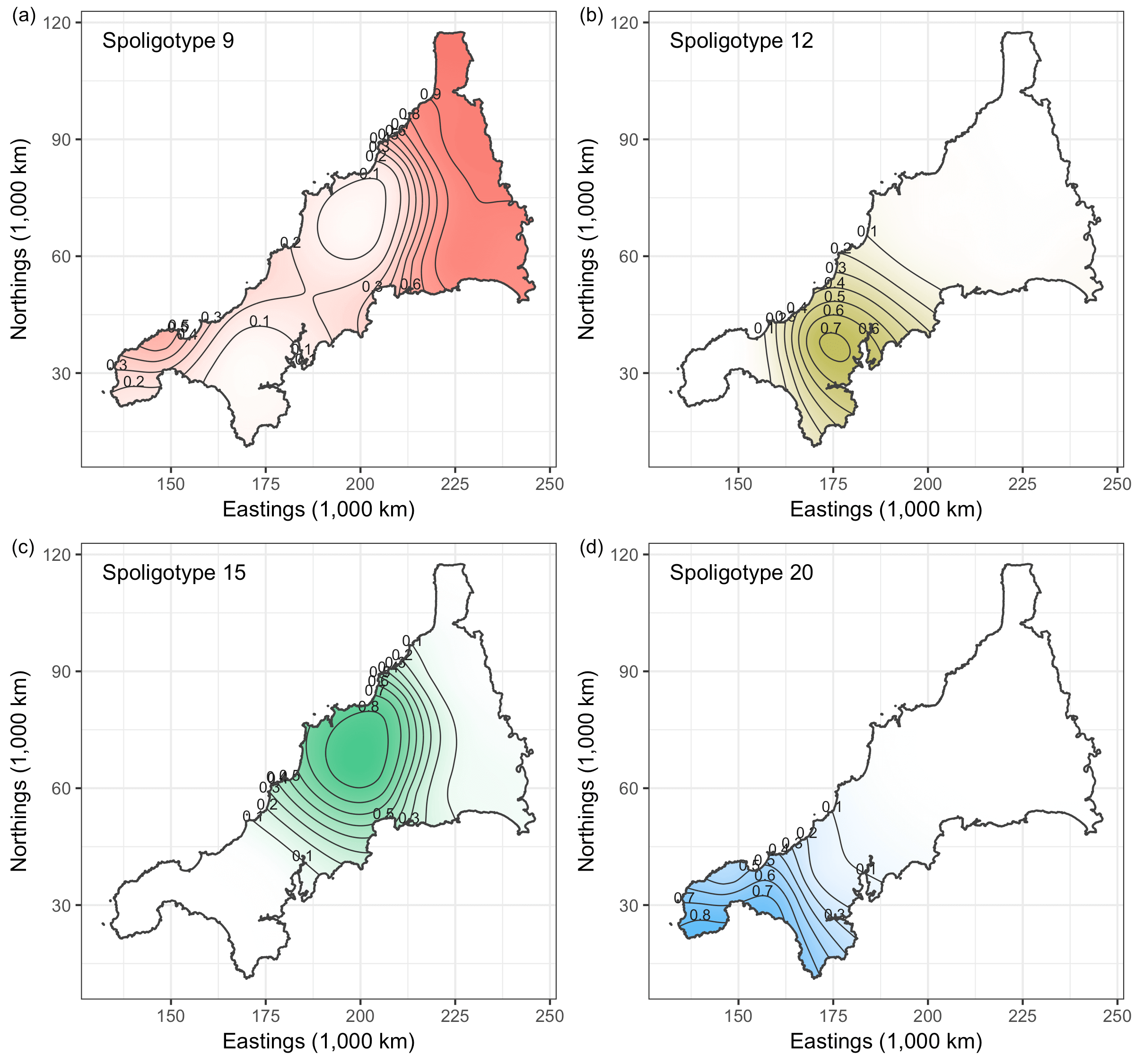
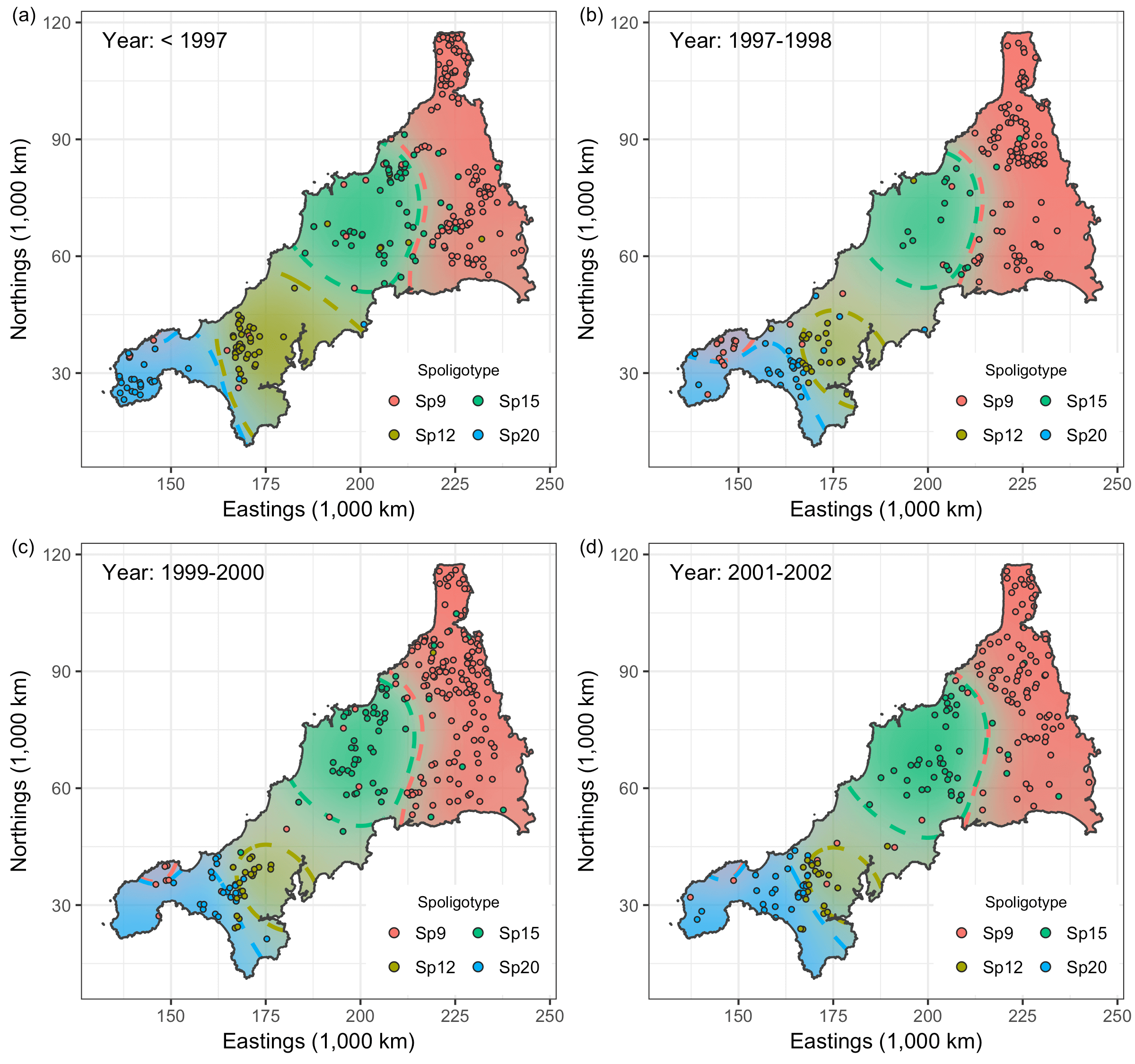
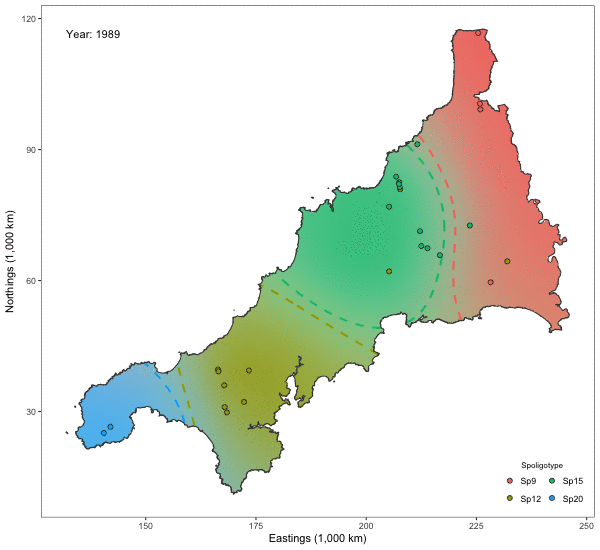
Spatio-temporal Analysis of Bovine Tubercolosis in Cornwall
Aim: Determine the existence of spatial segregation of multiple types of bovine tubercolosis (BTB) in Cornwall, and whether the spatial distribution had changed over time.
Data: Data pertaining to the location \(x_i\) (Northings and Eastings) and year of the occurrence \(t_i\). Nine hundred and nineteen cases of BTB had been recorded over a period of 14 years all over Cornwall. There are four types of BTB which are most commonly occurring, though a class of “others” was also considered totalling five classes.
Model: A multinomial I-probit model regressing the class probabilities on \(x_i\) and \(t_i\):
\[p_{ij} = g^{-1}_j \big( f_{1}(x_i) + f_{2}(t_i) + f_{12}(x_i,t_i) \big).\]A smooth effect of \(x_i\) is assumed, so \(f_{1j}\) lies in the fBm-0.5 RKHS. We have two choices for \(t_i\): 1) Assume a similar smooth effect; or 2) Aggregate the data into distinct time periods so that \(t_i\) emits a nominal effect (cf. the Pearson RKHS).
Results: The plots indicate that there is in fact spatial segregation between the various types of BTB in Cornwall. These can be tested formally by performing tests of significance on the scale parameters associated with location and time.