Classification with I-priors
The I-prior methodology is extended from the continuous response case to the categorical response case - we call this the I-probit model. Estimation involves some form of approximation as the marginal density cannot be found in closed form.
Categorical Responses
Suppose that each of the response variables \(y_i\) takes on one of the values from \(\{1,\dots,m\}\), and that
\[y_i \sim \text{Cat}(p_{i1}, \dots, p_{im})\]with probability mass function
\[p(y_i) = \prod_{j=1}^m p_{ij}^{y_{ij}}, \hspace{1cm} y_{ij} = [y_i = j]\]satisfying \(p_{ij} \geq 0\), and \(\sum_{j=1}^m p_{ij} = 1\).
The categorical distribution is a special case of the multinomial distribution, and can be seen as a generalisation of the Bernoulli distribution. Here, we have used the notation \([\cdot]\) to denote the Iverson bracket - \([A]\) equals one if the proposition \(A\) is true, and zero otherwise.
The assumption of normality on \(y_i\) is now highly inappropriate. In the spirit of generalised linear models, we model instead
\[\text{E}[y_{ij}] = p_{ij} = g^{-1}\big( f_j(x_{ij})\big)\]using some link function \(g:[0,1] \to \mathbb R\) and a regression function for each class \(j\), on which an I-prior is specified. As we will see later, the probit link \(g = \Phi^{-1}\) is preferred, where \(\Phi\) is the cumulative distribution function (CDF) for a standard normal distribution.
Binary Responses
In the simplest case where \(m=2\), each \(y_i\) follows a Bernoulli distribution with success probability \(p_i\). The probit link can be motivated through the use of continuous, underlying latent variables \(y_i^*,\dots,y_n^*\) such that
\[y_i = \begin{cases} 1 & \text{if } y_i^* \geq 0 \\ 0 & \text{if } y_i^* < 0. \\ \end{cases}\]We can then model these auxiliary random variables \(y_i^*\) using an I-prior as usual (cf. Model 1) with fixed error precision \(\Psi = I_n\). Thus,
\begin{align}
p_i = \text{P}(y_i = 1) &= \text{P}(y_i^* \geq 0) \nonumber \
&= \text{P}\big(f(x_i) + \epsilon_i \geq 0\big) \nonumber \
&= \Phi \big(f(x_i) \big). \nonumber
\end{align}
There is no loss of generality compared with using an arbitrary threshold \(\tau\) (other than zero) for the \(1\text{-}0\) determination or precision \(\Psi\) (other than identity) for the error terms \(\epsilon_i\).
Multinomial Responses
The approach we take is to model each probability class \(p_{ij}\) using separate regression functions \(f_j\) and separate I-priors (thus the index \(j\) on the functions). In the most general setting, there would be \(m\) sets of hyperparameters to estimate (one for each class), though it is possible to assume some common values among classes.
Using a latent variable motivation similar to the binomial case, we find that
\[\begin{align} p_{ij} = \text{E}_Z\Bigg[\mathop{\prod_{k=1}^m}_{k \neq j} \Phi\big(Z + f_j(x_i) - f_k(x_i)\big) \Bigg]. \tag{3} \end{align}\]For \(m > 3\) this is known not to have a closed-form expression, but nonetheless is easily evaluated using quadrature methods.
It is also possible to reparameterise the model by anchoring on one latent variable as the reference class and working with the latent differences so that only \(m − 1\) I-priors are required. It is easily seen that using this approach with \(m=2\) reduces the model to the same binomial model described above.
Estimation
Unlike the normal regression model, the marginal likelihood
\[p(\mathbf y) = \int \prod_{i=1}^n \prod_{j=1}^m \left[ \big\{ g^{-1}\big(f_j(x_i)\big) \big\}^{[y_i=j]} \cdot \text{N}_n (\mathbf{f}_{0j}, \mathcal I[f_j]) \, \text{d}\mathbf f_j \right],\]on which the posterior depends, is no longer available in closed form. Several methods can be employed to overcome this intractable integral, by way of approximating the true posterior density by \(q(\mathbf y)\), in order to obtain estimates of the hyperparameters. These are described below in an order analogous to the methods described in the normal regression model.
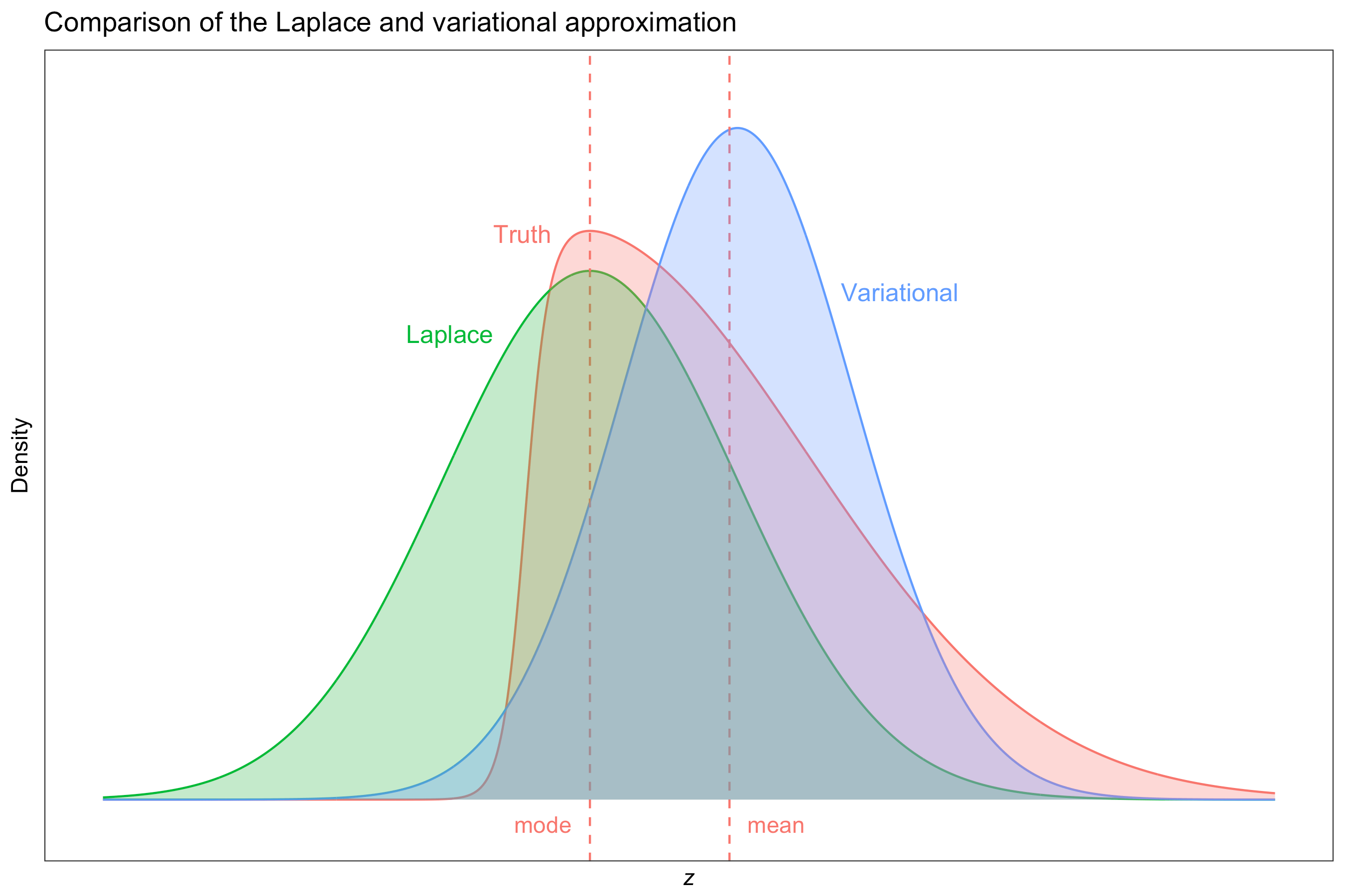
Laplace’s Method
Suppose that we are interested in
\[p(\mathbf f \vert \mathbf y) \propto p(\mathbf y \vert \mathbf f) p(\mathbf f) =: e^{Q(f)},\]with normalising constant \(p(\mathbf y) = \int e^{Q(f)} \, \text{d}\mathbf f\) (the marginal). The Taylor expansion of \(Q\) about its mode \(\mathbf f^*\),
\[Q(\mathbf f) \approx Q(\mathbf f^*) - \frac{1}{2} (\mathbf f - \mathbf f^*)^\top A (\mathbf f - \mathbf f^*),\]is recognised as the logarithm of an unnormalised Gaussian density, with \(A = -\text{D}^2 Q(\mathbf f^*)\) being the negative Hessian of \(Q\) evaluated at \(\mathbf f^*\). Therefore, the posterior density \(p(\mathbf f \vert \mathbf y)\) can be approximated by \(\text{N}_n(\mathbf f^*, A^{-1})\), and the marginal by
\[p(\mathbf y) \approx (2\pi)^{n/2} \vert A \vert^{-1/2} p(\mathbf y \vert \mathbf f^*) p(\mathbf f^*).\]The marginal density can then be maximised with respect to the hyperparameters using Newton-based methods. However, each Newton step would require finding the posterior modes \(\mathbf f^*\), which is difficult for very large \(n\).
Variational Approximation
An approximation \(q(\mathbf f)\) to the true posterior density \(p(\mathbf f \vert \mathbf y)\) is considered, with \(q\) chosen to minimise the Kullback-Leibler divergence (under certain restrictions),
\[\text{KL}(q || p) = - \int \log \frac{p(\mathbf f \vert \mathbf y)}{q(\mathbf f)} q(\mathbf f) \, \text{d}\mathbf f.\]The name “variational” stems from the fact that we are seeking to minimise a functional (the Kullback-Leibler divergence) which uses calculus of variations techniques. Of course it would be impossible to minimise the KL over all possible functions \(q\), so some restrictions are required. We use the mean-field factorisation assumption, which considers only densities which factorises completely over its components, i.e. densities of the form \(q(z_1, \dots, z_N) = \prod_{i=1}^N q(z_i).\)
By assuming priors on the hyperparameters \(\mathbf \theta\), we work in a fully Bayesian setting and append these model hyperparameters to \(\mathbf f\) to form \(\mathbf z = (\mathbf f, \mathbf \theta)\) and obtain a variational approximation to the posterior density \(p(\mathbf z \vert \mathbf y)\). The result is a sequential updating scheme similar to the EM algorithm.
This variational-EM algorithm works harmoniously with exponential family distributions, and as such the probit link provides an advantage over other link functions such as the more popular logit. In fact, all of the required posterior densities, with the exception of the \(y_i\), involve the normal distribution. The posterior distribution for \(y_i\) is of course categorical.
The marginal likelihood is approximated by a quantity known as the variational lower bound, and is given by \(\mathcal L = \text{E}_{\mathbf z}[\log p(\mathbf y, \mathbf z)] - \text{E}_{\mathbf z}[\log q(\mathbf z)]\), where expectation is taken over the approximate posterior distribution \(q\).
Markov Chain Monte Carlo
In keeping with the Bayesian theme, MCMC samplers such as Gibbs or Hamiltonian Monte Carlo can also be used to estimate these I-probit models. The MCMC method is a form of stochastic approximation which guarantees asymptotically exact results. However, in our experience, these methods can be computationally slow, and sampling difficulty often arises which result in unreliable posterior samples.
Modelling and Prediction
The advantages of I-priors in the normal model extend even to the I-probit model. This includes being able to simply model various types of categorical response regression models by choosing appropriate kernel functions for the covariates.
For prediction purposes, we can derive the posterior predictive class probabilities given a new data point \(x_\text{new}\) as follows:
\[\text{P}(y_\text{new} = j \vert \mathbf y) \approx \int \prod_{j=1}^m \Big[ p(y_{\text{new},j} \, \vert \, f_{\text{new},j}) q(f_{\text{new},j}) \, \text{d} f_{\text{new},j} \Big],\]where \(f_{\text{new},j} = f_j(x_\text{new})\) in which the approximate posterior density of \(q\) is used. This complex integral reduces to the expectation of products of standard normal CDFs (similar to 3).
For examples of I-probit models used for binary and multiclass classification, meta-analysis, and spatio-temporal modelling, see the Examples section.