Introducing I-priors

7 minute read

An introduction to regression with I-priors begins with a description of the regression model of interest and the definition of an I-prior. Some relevant reproducing kernel Hilbert spaces and also estimation methods for I-prior models are then described.

Introduction

Consider the following regression model for \(i=1,\dots,n\):

\begin{align} \begin{gathered} y_i = f(x_i) + \epsilon_i \
(\epsilon_1, \dots, \epsilon_n)^\top \sim \text{N}_n(0, \Psi^{-1}) \end{gathered} \end{align}

where each \(y_i \in \mathbb{R}\), \(x_i \in \mathcal{X}\), and \(f \in \mathcal{F}\). Here, \(\mathcal{X}\) represents the set of characteristics of unit \(i\), which may be numerical or nominal, uni- or multi-dimensional, or even functional.

Let \(\mathcal{F} \) be a reproducing kernel Hilbert space (RKHS) with kernel \(h: \mathcal{X} \times \mathcal{X} \to \mathbb{R} \). The Fisher information for \(f\) evaluated at two points \(x\) and \(x’\) is given by

\[\mathcal{I} \big( f(x), f(x') \big) = \sum_{k=1}^n \sum_{l=1}^n \Psi_{k,l} h(x,x_k) h(x', x_l).\]

The I-prior

The entropy maximising prior distribution for \(f\), subject to constraints, is

\[\mathbf{f} = \big(f(x_1), \dots, f(x_n) \big)^\top \sim \text{N}_n(\mathbf{f}_0, \mathcal{I}[f]) \]

where \(\mathbf{f}_0 = \big(f_0(x_1), \dots, f_0(x_n) \big)^\top\) is some prior mean, and \(\mathcal{I}[f]\) is the Fisher information covariance matrix with \((i,j)\)th entries given by \( \mathcal{I} \big( f(x_i), f(x_j) \big) \).

As such, an I-prior on \(f\) can also be written as

\begin{align} f(x) = f_0(x) + \sum_{i=1}^n h(x, x_i) w_i \end{align}

where \( (w_1,\dots,w_n)^\top \sim \text{N}_n(0, \Psi) \). Of interest then, are

the posterior distribution for the regression function
\[p(\mathbf{f}|\mathbf{y}) = \frac{p(\mathbf{y}|\mathbf{f})p(\mathbf{f})}{\int p(\mathbf{y}|\mathbf{f})p(\mathbf{f}) \, \text{d}\mathbf{f}} \text{; and}\]
the posterior predictive distribution given new data \(x_\text{new}\)
\[p(y_\text{new}|\mathbf{y}) = \int p(y_\text{new}|f_\text{new}, \mathbf{y}) p(f_\text{new} | \mathbf{y}) \, \text{d}f_\text{new}\]
where \(f_\text{new} = f(x_\text{new})\).

Reproducing Kernel Hilbert Spaces

Working in RKHSs gives us nice topologies, including being able to calculate the Fisher information for our regression function. In addition, it is well-known that there is a one-to-one bijection between the set of positive definite functions (i.e. kernels) and the set of RKHSs. Here are several kernels that are used for I-prior modelling.

The linear canonical kernel

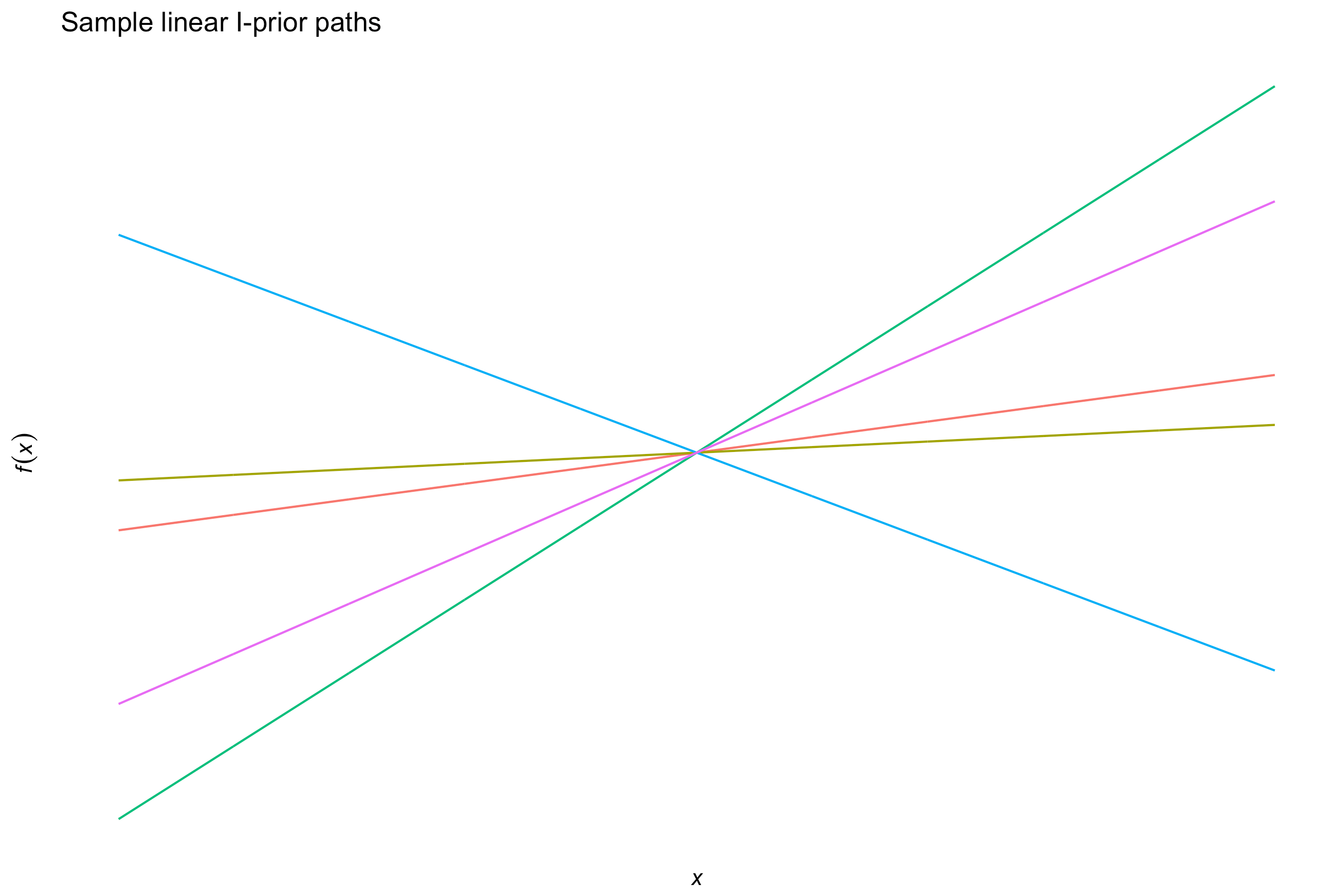
For \( x,x’ \in \mathcal{X} \),

\[h(x,x') = \langle x,x' \rangle_\mathcal{X}.\]

This kernel is typically used for real-valued covariates.

The fractional Brownian motion (fBm) kernel

Sample paths from the fBm kernel with varying Hurst coefficients.

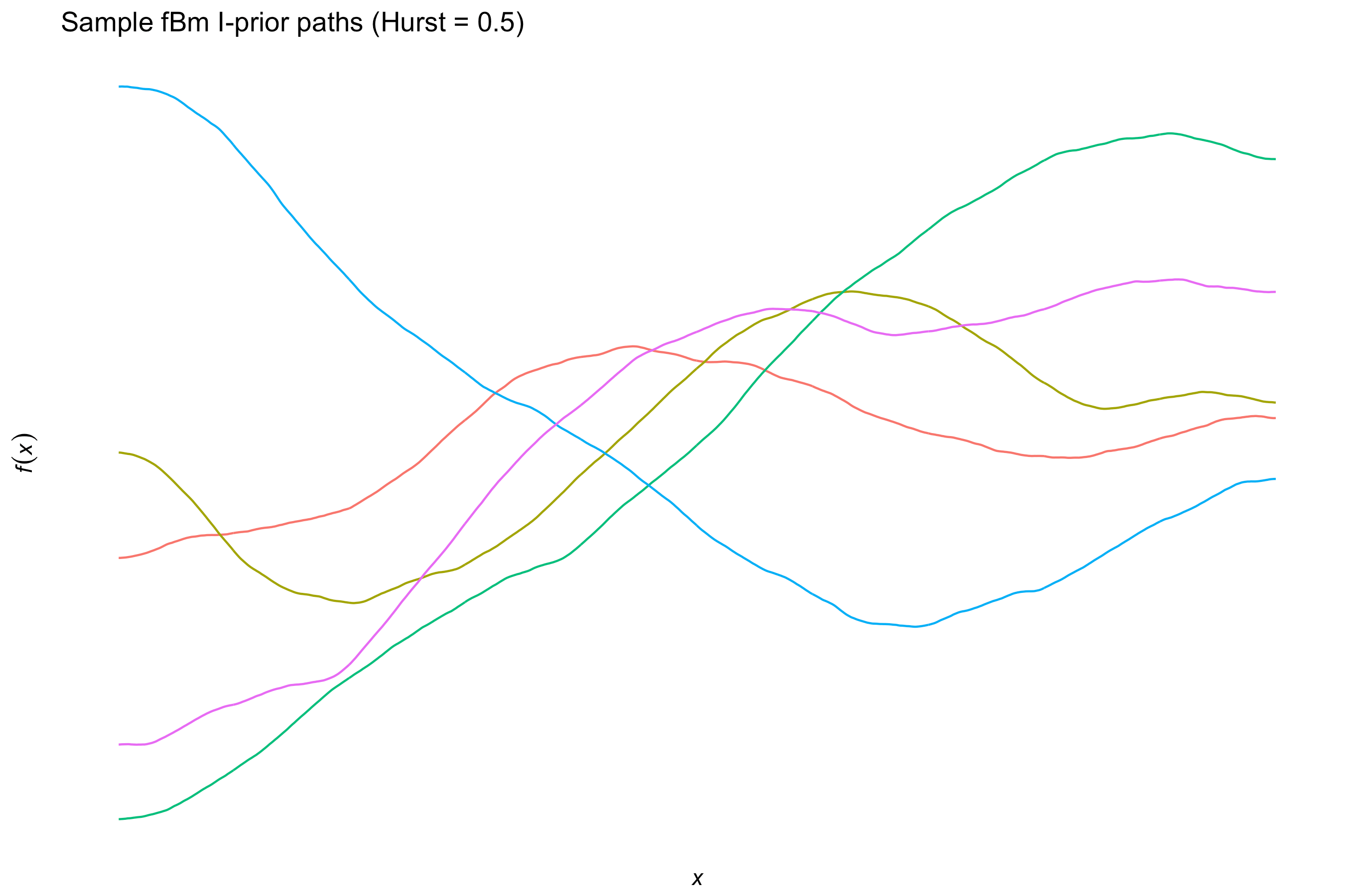
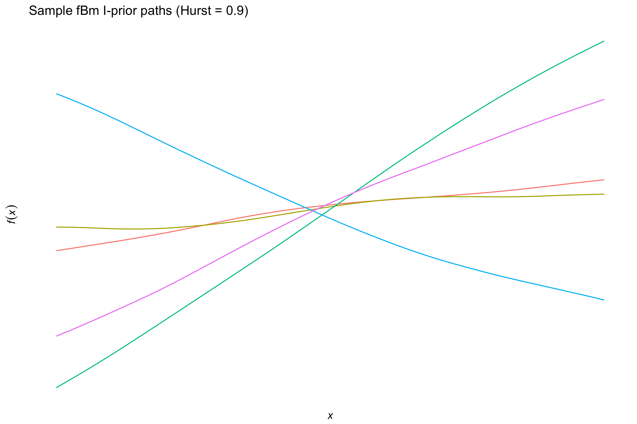
For \( x,x’ \in \mathcal{X} \),

\[h(x,x') = -\frac{1}{2} \left( \Vert x - x' \Vert^{2\gamma}_{\mathcal X} - \Vert x \Vert^{2\gamma}_{\mathcal X} - \Vert x' \Vert^{2\gamma}_{\mathcal X} \right),\]

where the Hurst coefficient \( \gamma \in (0,1) \) controls the smoothness of the fBm paths. Like the canonical kernel, this is also typically used for real-valued covariates.

The Pearson kernel

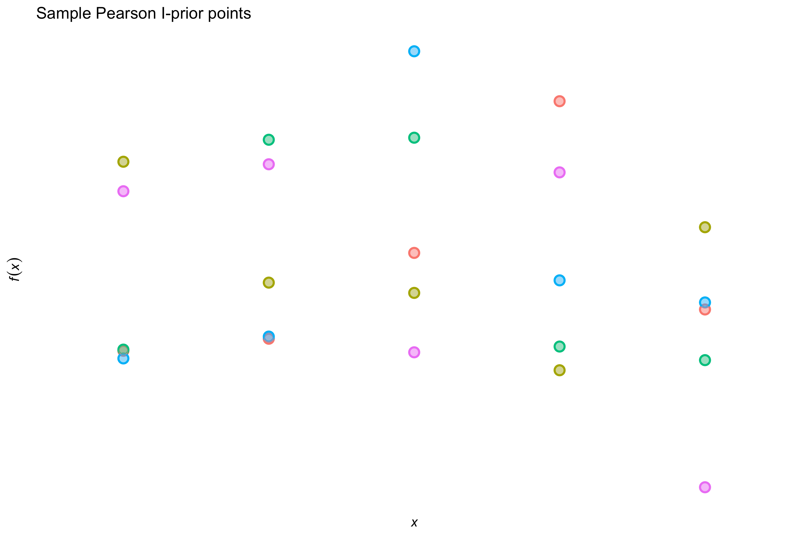
Let \( \mathcal{X} \) be a countably finite set, and let \(\text{P}\) be a probability distribution over it. Then,

\[h(x,x') = \frac{\delta_{xx'}}{\text{P}(X = x)} - 1,\]

where \(\delta\) is the Kronecker delta. This kernel is used for regression with nominal independent variables. The empirical distribution can be used in lieu of the true distribution \( \text{P} \).

Other kernels

Some other kernels include

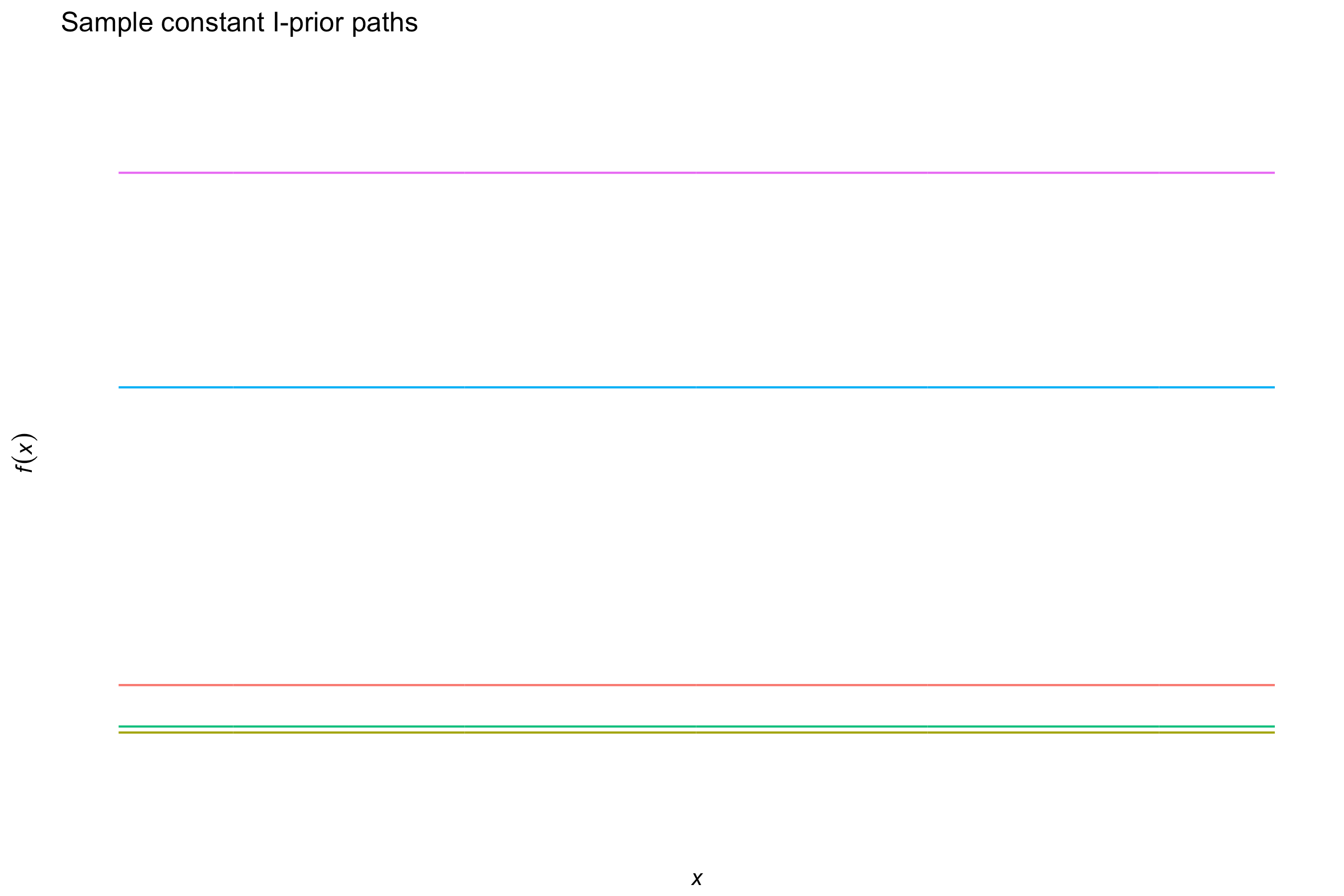
the (not-so-interesting-though-essential) constant kernel
\[h(x,x') = 1\]
for the RKHS of constant functions, which allow us to model an “intercept” effect;
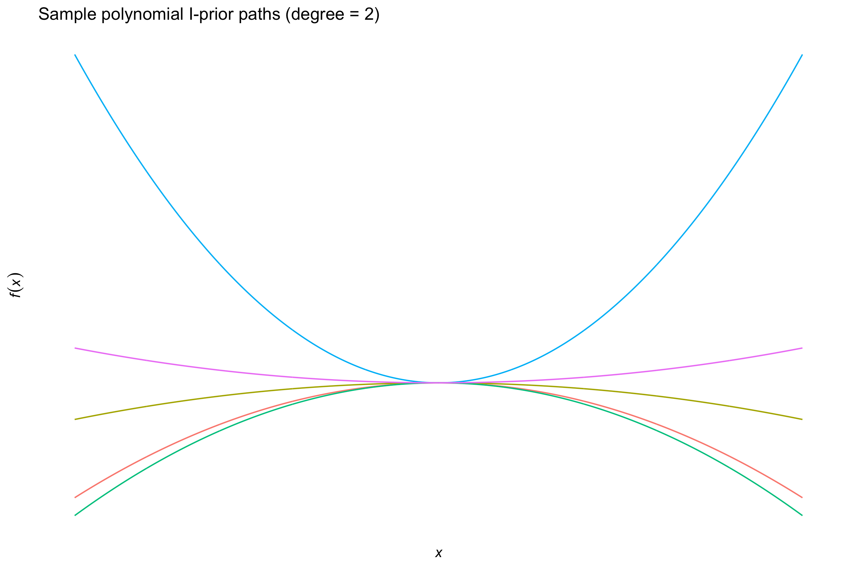
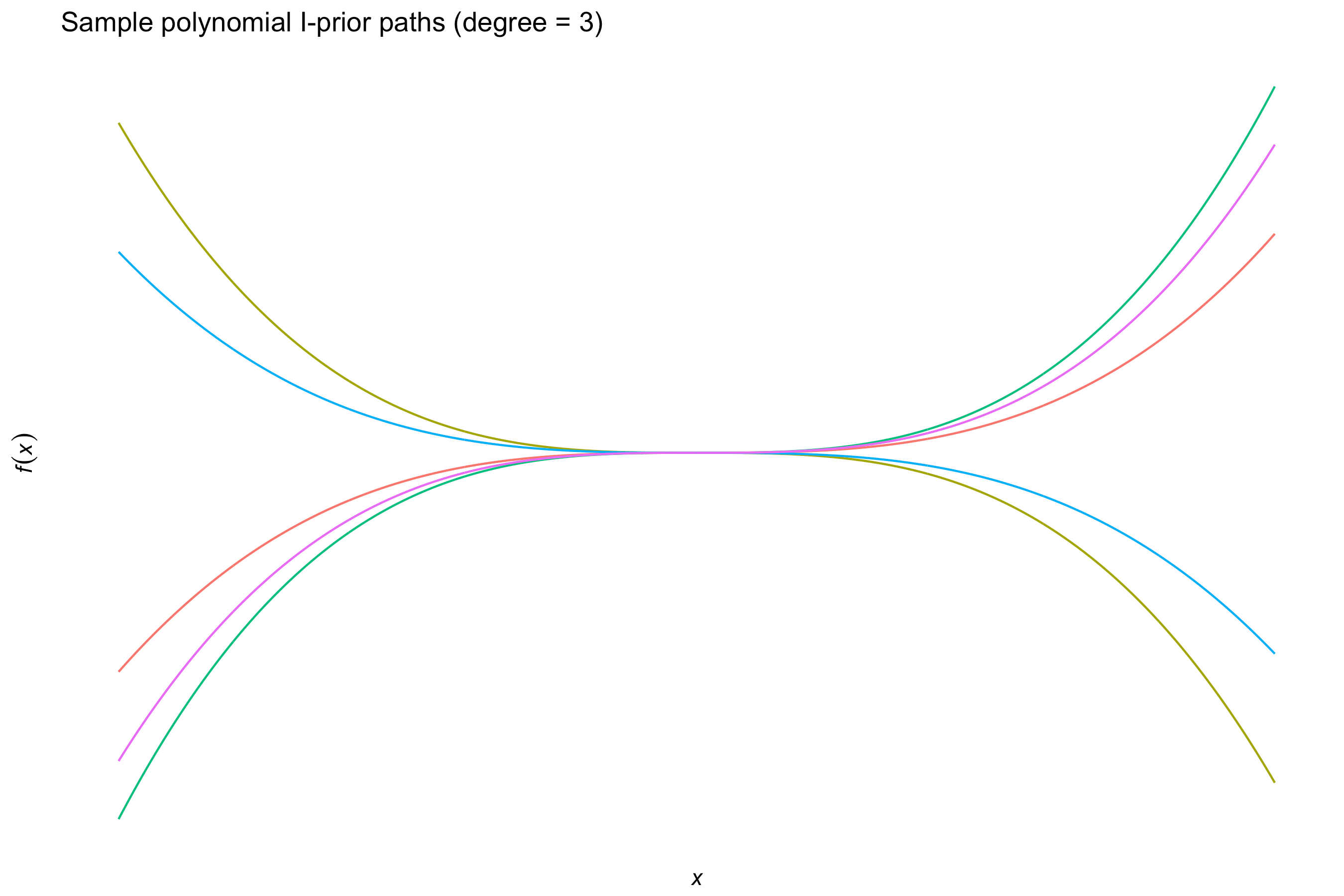
the \(d\)-degree polynomial kernel
\[h(x,x') = \big( \langle x,x' \rangle + c \big)^d\]
for some offest \(c \geq 0 \), which allow squared, cubic, quartic, etc. terms to be included easily; and
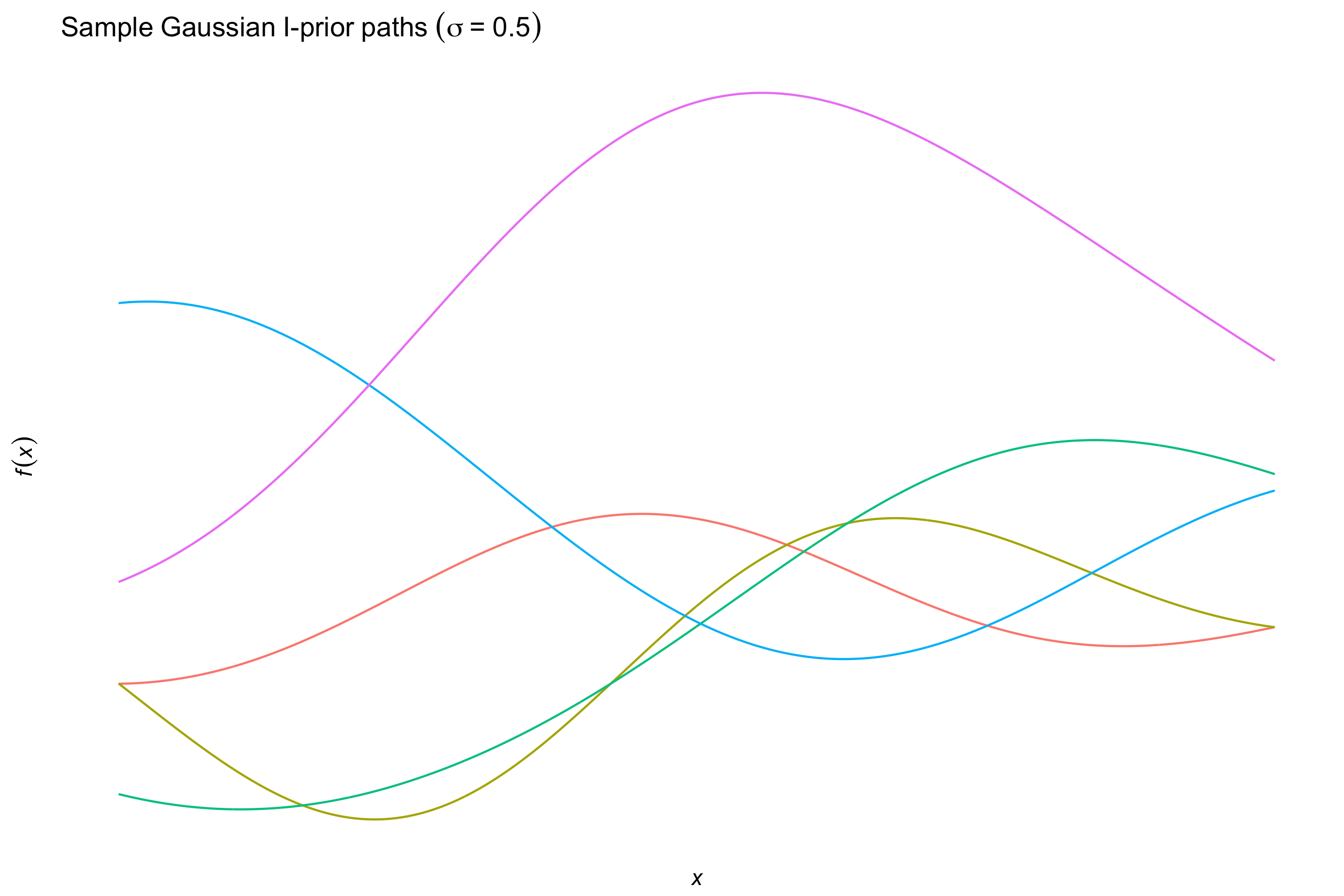
the squared exponential or Gaussian kernel
\[h(x,x') = \exp\left(-\frac{\Vert x - x' \Vert_{\mathcal X}^2}{2l^2} \right)\]
for some length scale \(l > 0\), which, while being the de facto kernel for Gaussian process regression, is too smooth for I-prior modelling and would tend to over-generalise the effects of the covariate.

The Sobolev-Hilbert inner product

Let \( \mathcal{X} \) represent a set of differentiable functions, and assume that it is a Sobolev-Hilbert space with inner product

\[\langle x,x' \rangle_\mathcal{X} = \int \dot{x}(t) \dot{x}'(t) \, \text{d}t.\]

Let \( z \in \mathbb{R}^T \) be the discretised realisation of the function \( x \in \mathcal{X} \) at regular intervals \(t=1,\dots,T\). Then

\[\langle x,x' \rangle_\mathcal{X} \approx \sum_{t=1}^{T-1} (z_{t+1} - z_t)(z_{t+1}' - z_t'),\]

so we can proceed with either the linear, fBm, or any other kernels which make use of inner products.

Scale Parameters and Krein Spaces

The scale of an RKHS \(\mathcal F\) over a set \(\mathcal X\) with kernel \(h:\mathcal X \times \mathcal X \to \mathbb R\) may be arbitrary, so scale parameters \(\lambda\) are introduced resulting in the RKHS \(\mathcal F_\lambda\) having kernel \(h_\lambda = \lambda\cdot h\). The unknown \(\lambda\) parameter(s) may be estimated in a variety of ways - see below.

As we will see later, kernels may be added and multiplied together resulting in new kernels which induce an RKHS. However, with scale parameters present, it is possible that the resulting kernel is no longer positive-definite, i.e. some of the scale parameters may be negative. It is rather capricious to restrict the sign of the scale parameters, and thus it is necessary to work with these (possibly) non-positive kernels and the generalisation of Hilbert spaces known as Krein spaces. The resulting vector space of interest is then the reproducing kernel Krein space (RKKS).

In a single scale parameter model, the sign of the scale parameter is not identified in the marginal likelihood. In this case, the scale parameter is fixed to the positive orthant.

Though it is not necessary to have an in-depth knowledge of RKHS/RKKS for I-prior modelling, the interested reader is invited to refer to some reading material.

Estimation

Under the normal model in (1) subject to the I-prior in (2), the posterior distribution for \(y\), given some \(x\) and model hyperparameters, is normal with mean

\[\hat y (x) = f_0(x) + \mathbf{h}_\lambda^\top(x) \Psi H_\lambda \big(H_\lambda \Psi H_\lambda + \Psi^{-1}\big)^{-1} \big(y - f_0(x) \big)\]

and variance

\[\hat\sigma^2_y (x) = \mathbf{h}_\lambda^\top(x) \big(H_\lambda \Psi H_\lambda + \Psi^{-1}\big)^{-1} \mathbf{h}_\lambda(x) + \nu_x,\]

where \(\mathbf{h}_\lambda^\top(x)\) is a vector of length \( n \) with entries \( h_\lambda(x,x_i) \) for \(i=1,\dots,n\), \(H_\lambda\) is the \(n \times n\) kernel matrix, and \(\nu_x\) is some term involving \(\mathbf h_\lambda^\top (x)\) and the prior variance and covariances between \(y\) at \(x\) and \(y_1, \dots, y_n\).

The model hyperparameters are the model error precision \(\Psi\), RKHS scale parameter(s) \(\lambda\), and possibly any other parameters associated with the kernel. There are various ways to estimate these, which are explained below.

In the most general case there are \(n(n+1)/2\) covariance parameters in \(\Psi\) to estimate. For simplicity, we may assume identical and independent (iid) error precisions, so that \(\Psi = \psi I_n\).

Maximum (marginal) likelihood

Also known as the empirical Bayes approach, the marginal likelihood can be obtained by integrating out the I-prior from the joint density as follows:

\[p(\mathbf y) = \int p(\mathbf y | \mathbf f) p(\mathbf f) \, \text{d} \mathbf f.\]

When both the likelihood and prior are Gaussian, the integral has a closed form, and we find that the marginal distribution for \(\mathbf y\) is also normal. The log-likelihood to be maximised is

\[\log L(\lambda, \Psi) = -\frac{n}{2} \log 2\pi - \frac{1}{2} \log \vert V_y \vert - \frac{1}{2} \big(y - f_0(x) \big)^\top V_y^{-1} \big(y - f_0(x) \big)\]

with \(V_y = H_\lambda \Psi H_\lambda + \Psi^{-1}\). This can be done, for example, using Newton-type methods. For very simple problems this is the fastest method, though it is susceptible to local optima and numerical issues.

Expectation-maximisation algorithm

By using the model parameterisation

\begin{align} \begin{gathered} y_i = f_0(x_i) + \sum_{k=1}^n h_\lambda(x_i, x_k) w_k + \epsilon_i \
(\epsilon_1, \dots, \epsilon_n)^\top \sim \text{N}_n(0, \Psi^{-1}) \
(w_1, \dots, w_n)^\top \sim \text{N}_n(0, \Psi) \end{gathered} \nonumber \end{align}

we can treat the “random effects” \(w_i\) as missing, and proceed with the EM algorithm. Both the full-data likelihood and the posterior distribution for the random effects are easily obtained due to normality, especially with an iid assumption on the error terms. For typical models, the M-step can be found in closed form, so the algorithm reduces to an iterative updating scheme which is numerically stable, albeit slow.

Markov chain Monte Carlo methods

We can employ a fully Bayesian treatment of I-prior models by assigning prior distributions to the hyperparameters \(\lambda\) and \(\Psi\). Gibbs-based methods can then be employed to sample from the posterior of these hyperparameters and obtain point estimates using statistics such as the posterior mean.

In our experience, many real and simulated data examples suffer from severe auto-correlations in the MCMC chains. This sampling inefficiency can be overcome by using sophisticated methods such as Hamiltonian Monte Carlo.

My PhD Project