Regression with I-priors

This section describes choosing appropriate functions depending on the desired effect of the covariates on the response variable. The output of an I-prior model is a posterior distribution for the regression function of interest. Some computational hurdles are also described.

A Unifying Methodology for Regression

One of the advantages of I-prior regression is that it provides a unifying methodology for a variety of statistical models. This is done by selecting one or several appropriate RKHSs for the regression problem at hand. Here we illustrate the fitting of several types of models based on the general regression model

\begin{align} \begin{gathered} y_i = f(x_i) + \epsilon_i \
(\epsilon_1, \dots, \epsilon_n)^\top \sim \text{N}_n(0, \Psi^{-1}) \
\end{gathered} \end{align}

and an I-prior on \(f \in \mathcal F\) (an RKHS).

Linear Regression

Fitted regression line for a linear model under an I-prior.

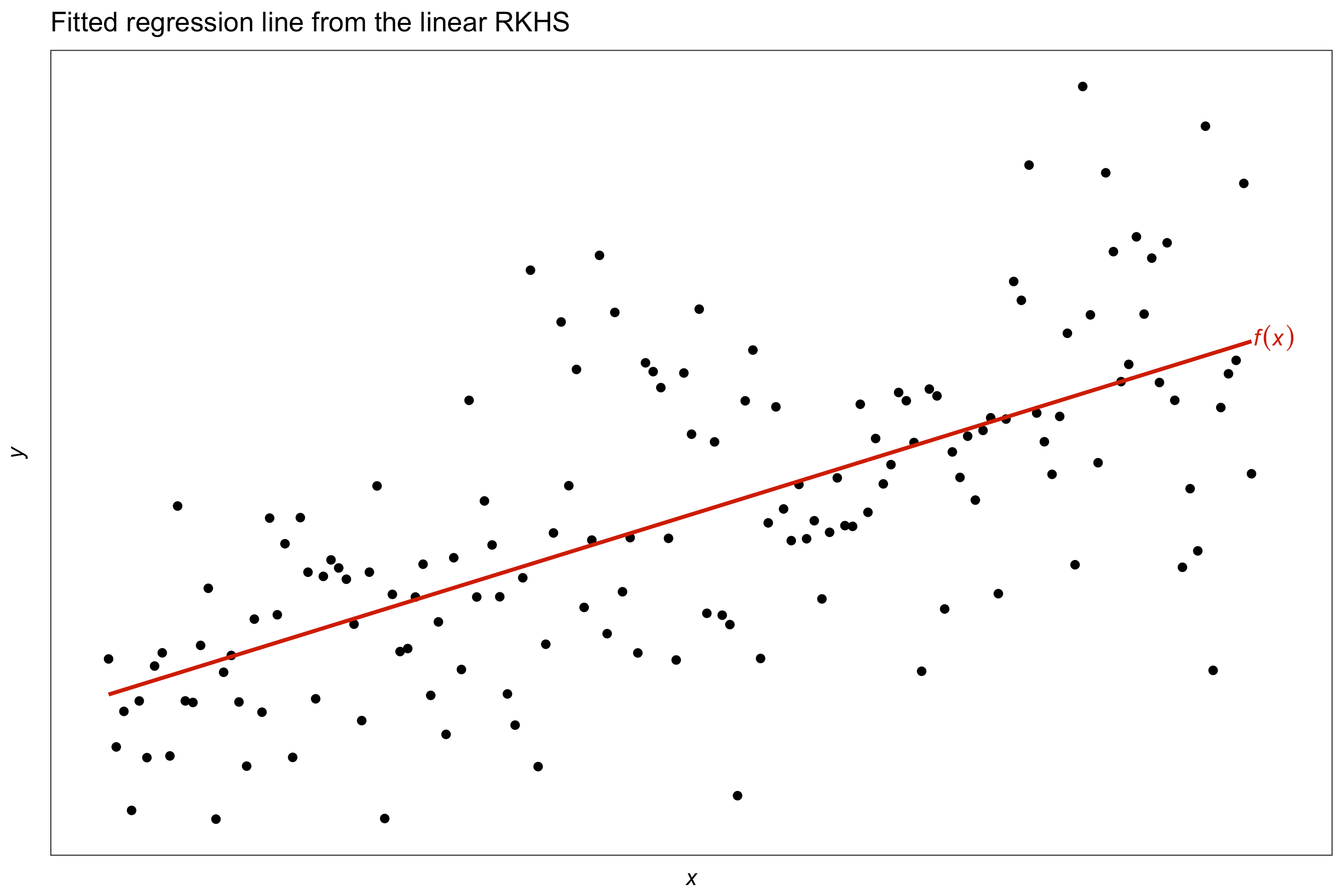
For simple linear regression, take \(\mathcal F\) to be the canonical linear RKHS with kernel \(h_\lambda = \lambda h\).

For multiple regression with \(p\) real-valued covariates, i.e. \(x_i = (x_{i1}, \dots, x_{ip})\), assume that

\[f(x) = f_1(x_{i1}) + \cdots + f_p(x_{ip})\]

where each \(f_j \in \mathcal F_j\), the canonical linear RKHS with kernel \(\lambda_j h_j\). The kernel

\[h_\lambda = \lambda_1 h_1 + \cdots + \lambda_p h_p\]

then defines the RKHS \(\mathcal F\).

Here we had assumed all covariates are real-valued. Any nominal valued covariate can be treated with the Pearson kernel instead. Also, higher order terms such as squared, cubic, etc. can be included by use of the polynomial kernel.

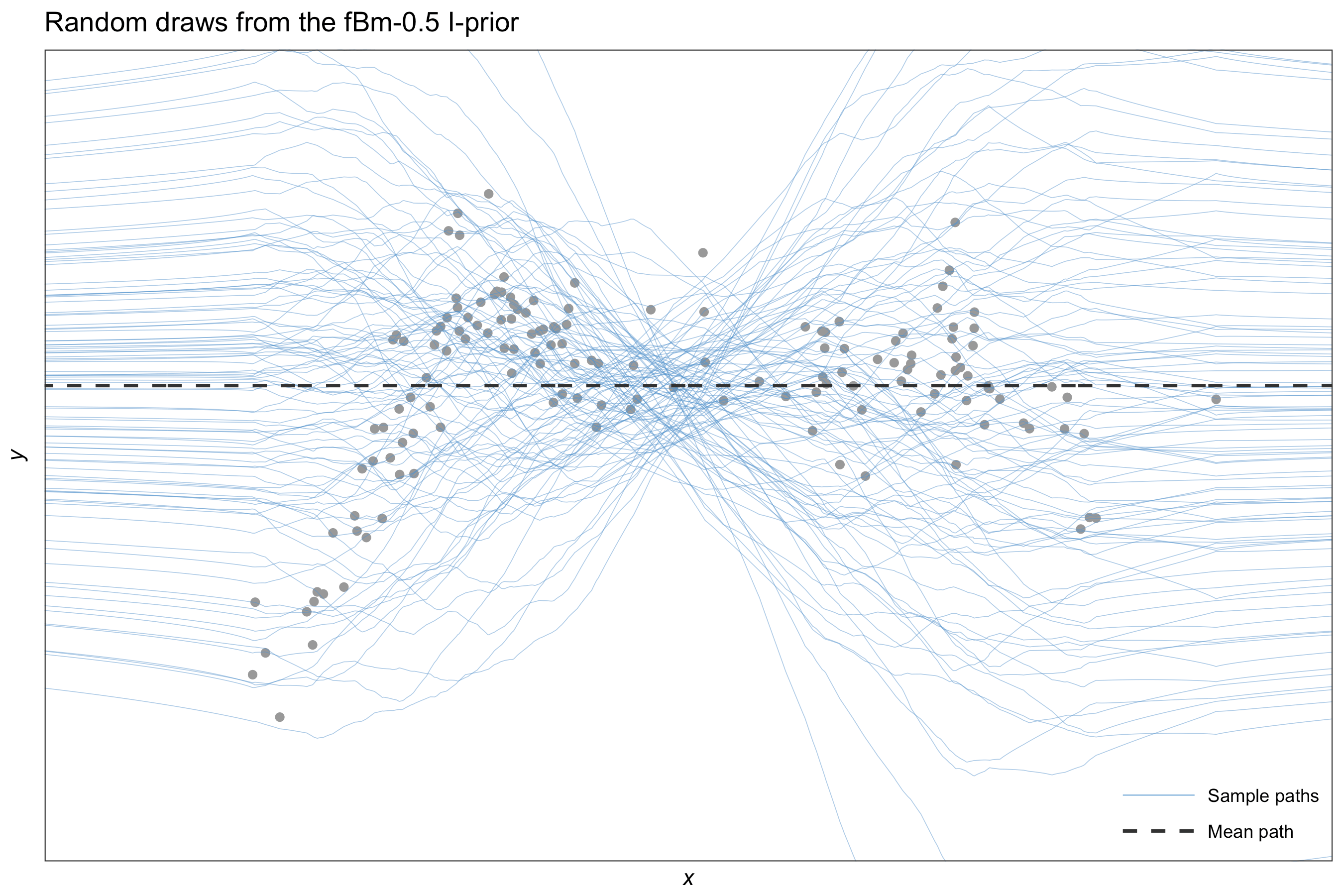
Smoothing Models

Fitted regression line for a smoothing model under an fBm I-prior.

Similar to the above, except that the fractional Brownian motion kernel is used instead. Other choices include the squared exponential kernel, or even the polynomial kernel with degree two or greater - though the fBm kernel is much preferred for I-prior smoothing.

Multilevel Models

Fitted regression line for a varying intercept model and a varying slope model under an I-prior.

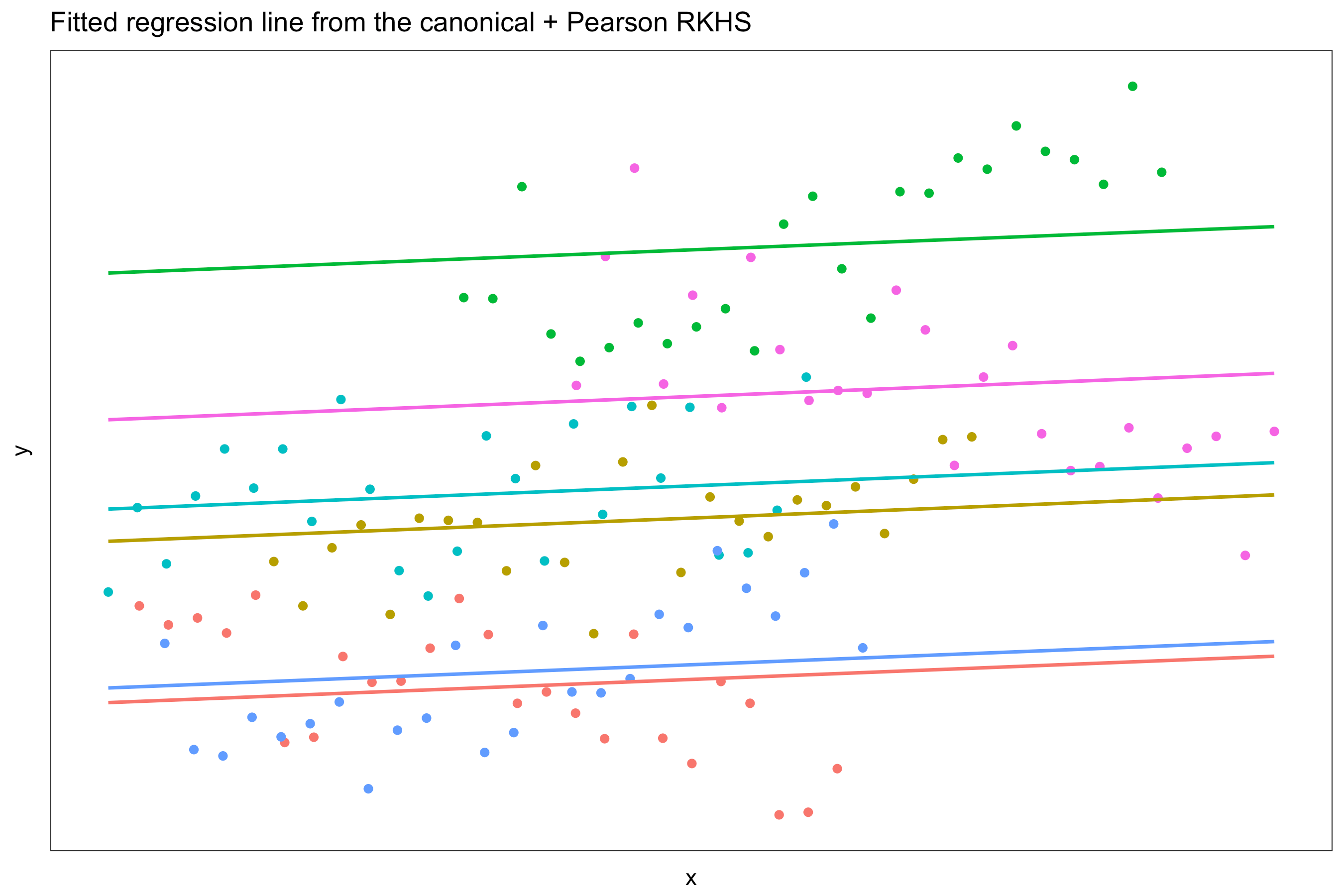
Suppose we had observations \(\{ (y_{ij}, x_{ij}) \}\) for each unit \(i\) in group \(j \in \{ 1,\dots,m \}\). We can model this using the function

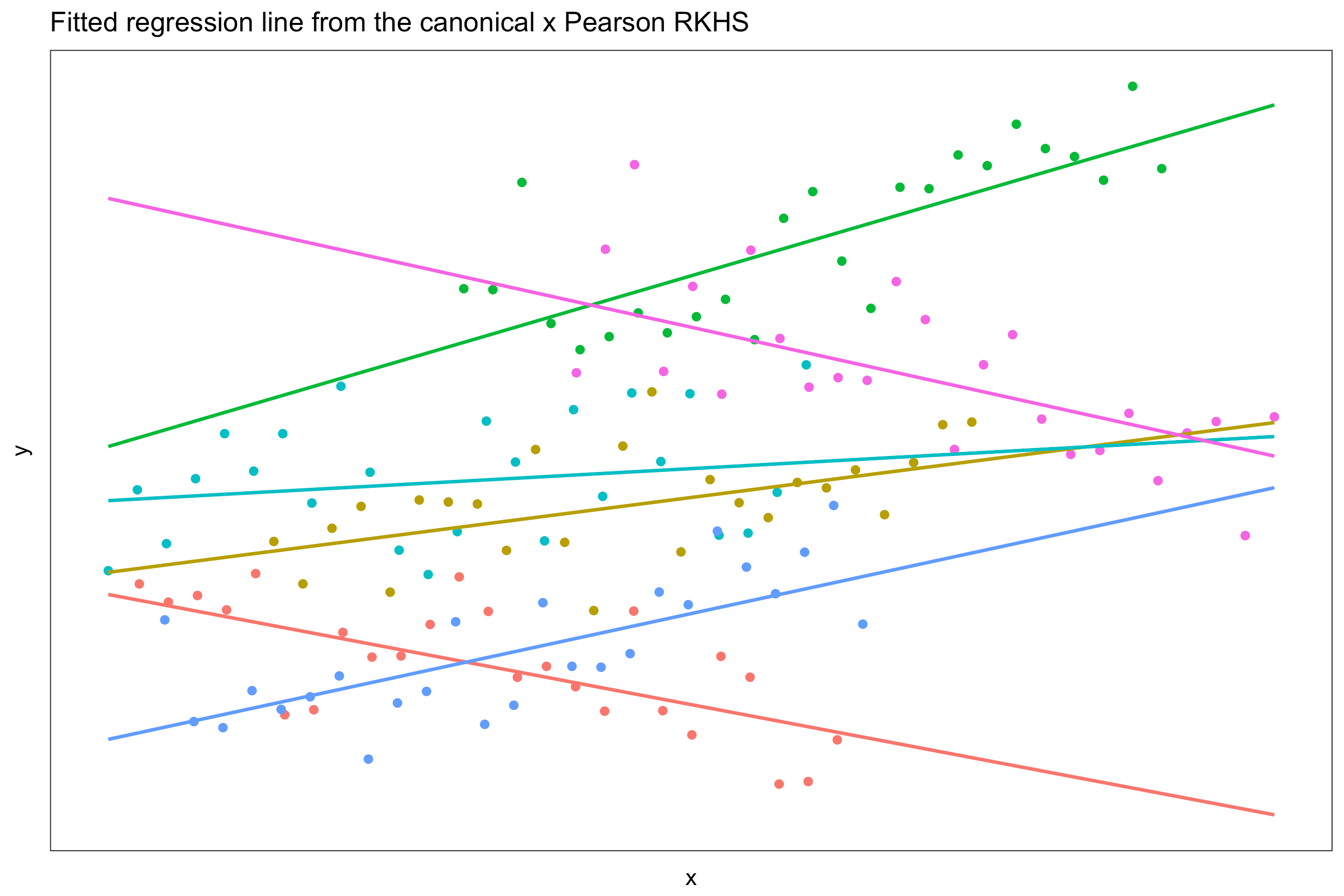
\[f(x_{ij}, j) = f_1(x_{ij}) + f_2(j) + f_{12}(x_{ij}, j).\]

Here we assume a linear effect on the covariates \(x_{ij}\) and a nominal effect on the groups. Thus, \(f_1 \in \mathcal F_1\) (linear RKHS) and \(f_2 \in \mathcal F_2\) (Pearson RKHS). Also assume that \(f_{12} \in \mathcal F_{12}\), the so-called tensor product \(\mathcal F_1 \otimes \mathcal F_2\). The kernel given by

\[h_\lambda = \lambda_1 h_1+ \lambda_2 h_2 + \lambda_1\lambda_2 h_1 h_2\]

defines the reproducing kernel for \(\mathcal F\). This gives results similar to a varying slopes model, while the model without the “interaction” effect \(f_{12}\) gives results similar to a varying intercept model.

The I-prior method estimates only three parameters - two RKHS scale parameters and the error precision. Standard multilevel models estimate at most six - two intercepts, three variances, and one covariance, all the while needing to ensure positive definiteness is adhered to.

Longitudinal Models

Now suppose we had observations \(\{ (y_{it}, x_{it}) \}\) for each unit or individual \(i\) measured at time \(t \in \{ 1,\dots,T \}\). We have several choices for a model, such as modelling responses over time only:

\begin{align} f(x_{it}, t) = f(t) \nonumber \end{align}

or including \(x_{it}\) as an explanatory variable:

\begin{align} f(x_{it}, t) = f_1(x_{it}) + f_2(t) + f_{12}(x_{it}, t), \nonumber \end{align}

which would then be similar to the multilevel model, except that we don’t necessarily have to assume a nominal effect of time. We can instead choose either a linear or smooth effect of time by choosing the canonical or fBm RKHS respectively for \(f_2\).

Note that the interaction effect between time and the explanatory variable \(f_{12}\) need necessarily be present to model longitudinal effects. Otherwise, this would mean that explanatory variables has no time-varying effect.

Models with Functional Covariates

By considering the functional covariates to be in a Sobolev-Hilbert space of continuous functions, we can apply either the linear kernel or fBm kernel on the discretised first differences, similar to a linear or smoothing model.

Posterior Regression Function

Working in a Bayesian framework allows us to draw sample functions from the prior and posterior, obtain credibility intervals, and perform posterior predictive checks.

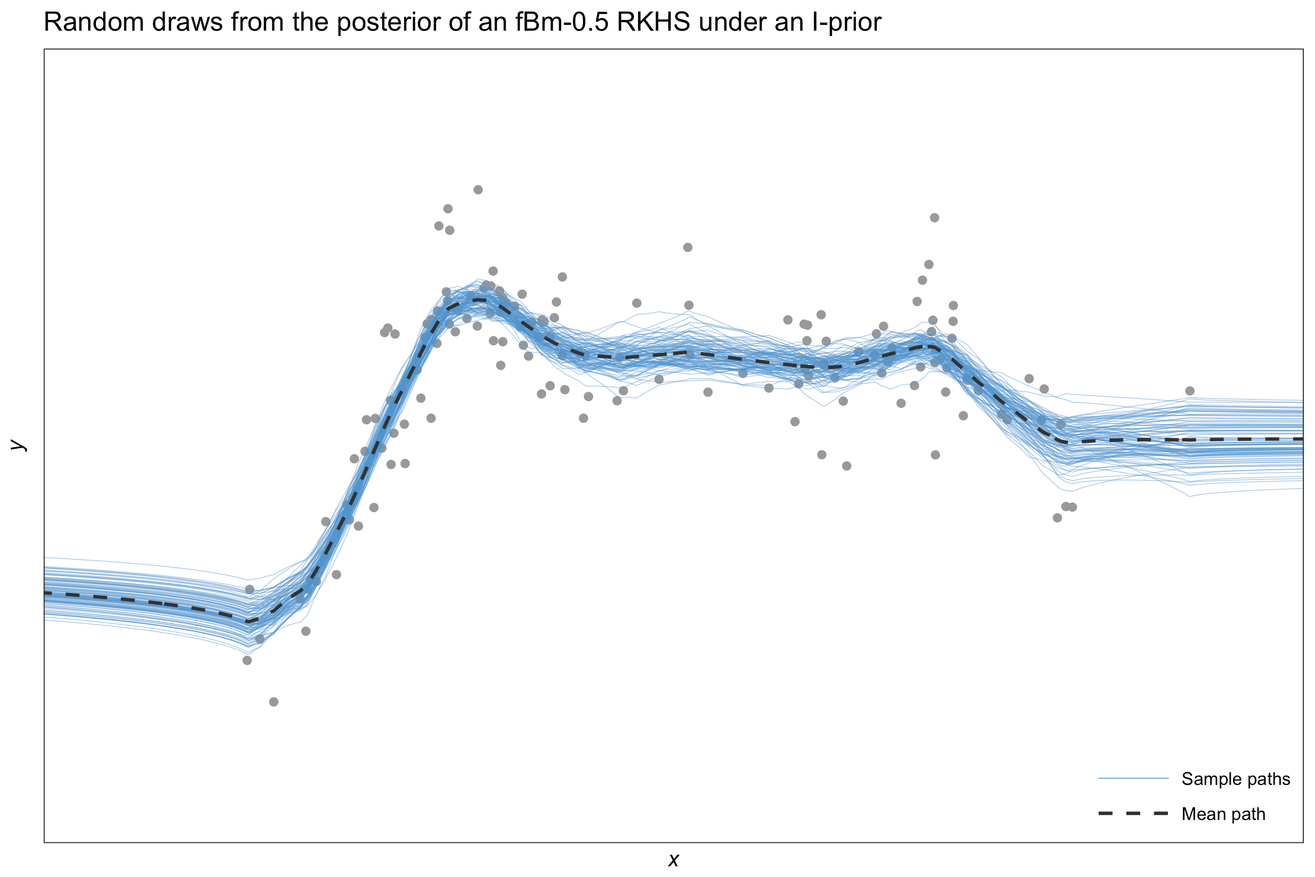
Estimation methods described in the Introduction page yields a posterior distribution for our regression function \(f(x)\) which is normally distributed with mean

\[\hat f (x) = f_0(x) + \mathbf{h}_\lambda^\top(x) \Psi H_\lambda \big(H_\lambda \Psi H_\lambda + \Psi^{-1}\big)^{-1} \big(y - f_0(x) \big)\]

and variance

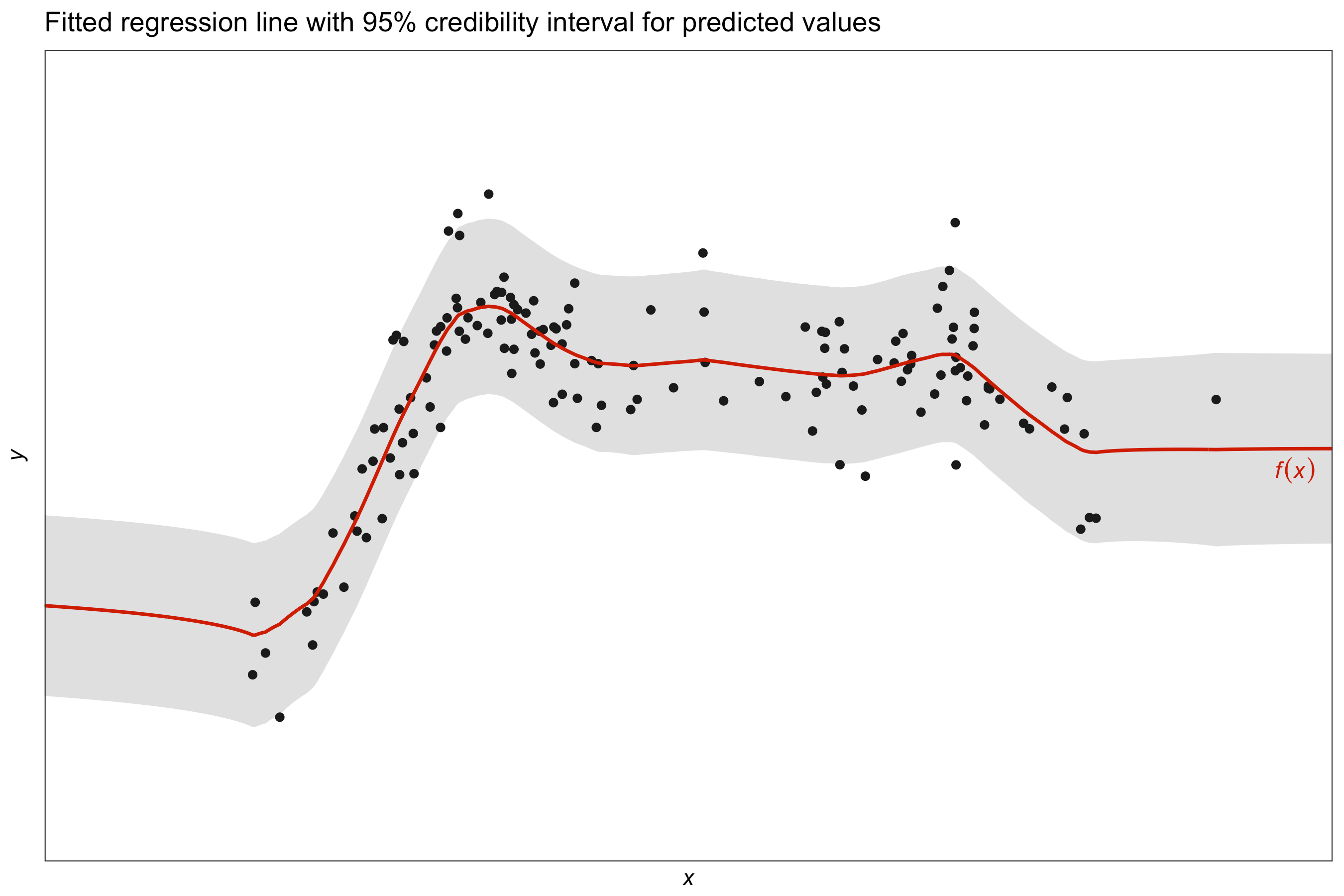
\[\hat{\sigma}^2_f (x) = \mathbf{h}_\lambda^\top(x) \big(H_\lambda \Psi H_\lambda + \Psi^{-1}\big)^{-1} \mathbf{h}_\lambda(x).\]

The posterior mean \(\hat f (x)\) can then be taken as a point estimate for \(f(x)\), the evaluation of the function \(f\) at a point \(x\). As this has a distribution, we can also obtain credible intervals for the estimate. The equation defining \(\hat{\sigma}^2_f\) can also be used to obtain the covariance between two points \(f(x)\) and \(f(x')\).

The posterior mean \(\hat f(x)\) is the same as the posterior mean \(\hat y(x)\) for a prediction \(y\) at a point \(x\), but the posterior variance \(\hat \sigma_f (x)\) is slightly different.

Computational Hurdles

Computational complexity is dominated by an \(n \times n\) matrix inversion which is \(O(n^3)\). In the case of Newton-based approaches, this needs to be evaluated at each Newton step. In the case of the EM algorithm, every update cycle involves such an inversion. For stochastic MCMC sampling methods, the inversion occurs in each sampling step.

Suppose that \(H_\lambda = QQ^\top\), with \(Q\) an \(n \times q\) matrix, is a valid low-rank decomposition. Then

\[\big(H_\lambda \Psi H_\lambda + \Psi^{-1}\big)^{-1} = \Psi - \Psi Q \big((Q^\top \Psi Q)^{-1} + Q^\top \Psi Q \big)^{-1} Q^\top\Psi,\]

obtained via the Woodbury matrix identity, is a much cheaper \(O(nq^2)\) operation, especially if \(q \ll n\).

Storage requirements for I-prior models are of \(O(n^2)\).

Canonical Kernel Matrix

Under the canonical linear kernel, the kernel matrix is given by

\[H_\lambda = X \Lambda X^\top,\]

where \(X\) is the \(n \times p\) design matrix of the covariates, and \(\Lambda\) \(=\) \(\text{diag}(\lambda_1, \dots, \lambda_p)\) is the diagonal matrix of RKHS scale parameters. The rank of \(H_\lambda\) is at most \(p\), and typically \(p \ll n\) so any algorithm for estimating the I-prior model can be done in \(O(np^2)\) time instead.

The Nyström Method

In other cases, such as under the fBm kernel, the matrix \(H_\lambda\) is full rank. Partition the kernel matrix as

\[H_\lambda = \begin{pmatrix} A_{m,m} &B_{m,n-m} \\ B_{m,n-m}^\top &C_{n-m,n-m} \\ \end{pmatrix}.\]

The Nyström methods provides an approximation to \(C\) by manipulating the eigenvectors and eigenvalues of \(A\) together with the matrix \(B\) to give

\[H_\lambda \approx \begin{pmatrix} V \\ B^\top V U^{-1} \\ \end{pmatrix} U \begin{pmatrix} V &B^\top V U^{-1} \\ \end{pmatrix}\]

where \(U\) is the diagonal matrix containing the \(m\) eigenvalues of \(A\), and \(V\) is the corresponding matrix of eigenvectors. An orthogonal version of this approximation is of interest, and can be achieved in \(O(2m^3)\). Estimation of I-prior models using the Nyström method takes \(O(nm^2)\) time and \(O(nm)\) storage, which is beneficial if \(m \ll n\).

There are many methods describing how to partition \(H_\lambda\), but it can be done as simply as randomly sampling \(m\) rows/columns without replacement to form the matrix \(A\). This method works well in practice.